Chapter 9: Inference Optimization
Inference Optimization: Making AI Models Better, Cheaper, and Faster
New models come and go, but one constant remains: the need to make them better, cheaper, and faster. While training models captures headlines, inference accounts for up to 90% of machine learning costs for deployed AI systems. If you're building production AI applications, understanding inference optimization isn't optional—it's essential.
Training vs. Inference: Two Sides of AI
An AI model's lifecycle has two distinct phases:
Training: Building the model through iterative learning
Inference: Using the trained model to compute outputs for given inputs
Unless you're training or finetuning models, you'll spend most of your time optimizing inference. In production, the component running model inference is called an inference server—it allocates resources based on application requests (like user prompts) and returns responses.
Understanding Computational Bottlenecks
Optimization fundamentally involves identifying bottlenecks and addressing them. Two main computational bottlenecks dominate inference:
Compute-Bound Operations
These tasks are limited by the raw computational power available. Their completion time depends on how many calculations the hardware can perform. Think of it as being constrained by how fast your processor can crunch numbers.
Memory Bandwidth-Bound Operations
These tasks are constrained by data transfer rates—how quickly data moves between memory and processors. If you store data in CPU memory but train on GPUs, the data transfer becomes a significant bottleneck. This limitation often manifests as the dreaded OOM (out-of-memory) error that engineers everywhere recognize.
The Two-Phase Dance of Language Model Inference
For transformer-based language models, inference consists of two distinct steps:
Prefill Phase: The model processes input tokens in parallel. How many tokens can be processed simultaneously depends on your hardware's operational capacity. This phase is compute-bound—limited by processing power.
Decode Phase: The model generates output tokens one at a time. This involves loading large matrices (model weights) into GPUs, constrained by how quickly hardware loads data into memory. This phase is memory bandwidth-bound—limited by data movement speed.
This distinction is crucial because these phases require fundamentally different optimization strategies.
Inference APIs: Online vs. Batch
Most providers offer two types of inference APIs, each optimized for different priorities:
Online APIs optimize for latency. Requests are processed immediately as they arrive. Customer-facing applications like chatbots and code generation require this low-latency approach for acceptable user experience.
Batch APIs optimize for cost and throughput. Multiple requests are processed together, sacrificing immediate response for efficiency. This works well for non-interactive workloads.
The key insight: online APIs focus on lower latency, batch APIs focus on higher throughput.
Critical Performance Metrics
Before optimizing anything, you need to measure what matters. Here are the essential metrics:
Latency Metrics
Overall Latency: Time from query submission to complete response delivery.
For streaming responses, latency breaks down into:
Time to First Token (TTFT): How quickly the first token appears after a user sends a query. This heavily influences perceived responsiveness.
Time Per Output Token (TPOT): How quickly each subsequent token generates after the first. If each token takes 100ms, a 1,000-token response takes 100 seconds.
Time Between Tokens (Inter-Token Latency): The gap between consecutive output tokens. Total latency equals: TTFT + (TPOT × number of output tokens).
Consider a scenario where the model generates an internal plan, takes actions, and logs outputs before showing the final response to users. The visible latency differs from total processing time—understanding this distinction matters for user experience optimization.
Throughput and Goodput
Throughput measures output tokens per second across all users and requests. Since prefilling and decoding have different computational bottlenecks and are often decoupled in modern inference servers, input and output throughput should be counted separately. When unspecified, "throughput" typically refers to output tokens.
Higher throughput generally means lower cost. Total cost per request combines prefilling and decoding costs. Smaller models and higher-end chips typically deliver higher throughput.
The classic trade-off: techniques like batching improve throughput but can reduce latency.
Goodput measures requests per second that satisfy your SLO (Service Level Objective). Unlike raw throughput, goodput focuses on quality—only successful requests meeting requirements count.
Utilization Metrics
GPU Utilization: Percentage of time the GPU actively processes tasks.
Model FLOP/s Utilization (MFU): The ratio of observed throughput (tokens/s) to theoretical maximum throughput at peak FLOP/s. This distinguishes practical performance from NVIDIA's GPU utilization metric.
Model Bandwidth Utilization (MBU): Percentage of achievable memory bandwidth used. If a chip's peak bandwidth is 1 TB/s but your inference uses only 500 GB/s, your MBU is 50%.
The pattern: Compute-bound workloads show higher MFU and lower MBU, while bandwidth-bound workloads show lower MFU and higher MBU.
For inference, prefill (compute-bound) typically shows higher MFU than decode (memory bandwidth-bound).
A critical insight: higher utilization means nothing if cost and latency both increase. What matters is getting jobs done faster and cheaper.
AI Accelerators: The Hardware Foundation
Software speed and cost depend fundamentally on underlying hardware. An accelerator is a chip designed for specific computational workloads. AI accelerators are optimized for AI tasks, with GPUs dominating the landscape.
CPUs vs. GPUs: Fundamental Differences
CPUs are designed for general-purpose usage with a few powerful cores (typically up to 64 for high-end consumer machines). They excel at tasks requiring high single-thread performance—running operating systems, managing I/O operations, handling complex sequential processes.
GPUs contain thousands of smaller, less powerful cores optimized for tasks that break down into many smaller, independent calculations like graphics rendering and machine learning. Matrix multiplication—the operation constituting most ML workloads—is highly parallelizable, making GPUs ideal.
Training vs. Inference Hardware
Training and inference have different hardware requirements:
Training demands much more memory due to backpropagation and is generally more difficult to perform in lower precision. Training emphasizes throughput.
Inference aims to minimize latency. Chips designed for inference are often optimized for lower precision and faster memory access rather than large memory capacity. Examples include Apple Neural Engine, AWS Inferentia, and Meta's MTIA (Meta Training and Inference Accelerator).
Edge computing chips like Google's Edge TPU and NVIDIA Jetson Xavier are also geared toward inference. Some chips specialize in specific architectures—for instance, chips optimized specifically for transformers.
Evolution of Compute Primitives
Different hardware architectures have different memory layouts and specialized compute units optimized for specific data types: scalars, vectors, or tensors.
GPUs traditionally supported vector operations, but modern GPUs now include tensor cores optimized for matrix and tensor computations.
TPUs (Tensor Processing Units) are designed with tensor operations as their primary compute primitive from the ground up.
To efficiently operate a model on any hardware architecture, you must consider its memory layout and compute primitives.
Key Hardware Characteristics
When evaluating chips, three main characteristics matter across use cases:
Computational Capabilities: Typically measured in FLOP/s (floating-point operations per second)—how many operations a chip performs in a given time.
Memory Size and Bandwidth: Because GPUs have many cores working in parallel, data constantly moves from memory to cores, making transfer speed critical. GPU memory requires higher bandwidth and lower latency than CPU memory, necessitating advanced memory technologies. This is why GPU memory costs more than CPU memory.
Three memory tiers matter:
CPU Memory (DRAM): Accelerators typically deploy alongside CPUs, accessing CPU memory
GPU High-Bandwidth Memory (HBM): Dedicated GPU memory located close to the GPU for faster access, with transfer speeds from 256 GB/s to over 1.5 TB/s
GPU On-Chip SRAM: Integrated directly into the chip for frequently accessed data, including L1/L2 caches (and sometimes L3)
Power Consumption: Chips rely on transistors for computation. Each computation requires transistors switching on and off, consuming energy. Power efficiency directly impacts operational costs and environmental impact.
Model-Level Optimization
Model-level optimization aims to make models more efficient, often by modifying the model itself, which can alter behavior. Language models have three characteristics making inference resource-intensive: model size, autoregressive decoding, and the attention mechanism.
Model Compression
Model compression reduces a model's size, often making it faster too.
Quantization: Reduces precision to shrink memory footprint and increase throughput. For example, moving from 32-bit floating-point to 8-bit integers dramatically reduces memory requirements while maintaining acceptable accuracy.
Model Distillation: Trains a smaller model to mimic a larger model's behavior. The student learns from the teacher's outputs, often achieving comparable performance with significantly fewer parameters.
Pruning: Has two meanings in neural networks. One removes entire nodes, changing architecture and reducing parameters. The other identifies parameters least useful for predictions and sets them to zero, making the model more sparse. This reduces storage space and speeds up computation.
Overcoming the Autoregressive Bottleneck
Autoregressive language models generate one token after another. If generating one token takes 100ms, a 100-token response takes 10 seconds. This process isn't just slow—it's expensive. Improving autoregressive generation by even a small percentage significantly enhances user experience.
Speculative Decoding (also called speculative sampling): Uses a faster but less powerful model to generate a sequence of tokens, which the target model then verifies. If the target model accepts the tokens, multiple tokens are generated in one pass. If not, it falls back to standard generation. This can substantially reduce generation time when the draft model produces acceptable tokens.
Inference with Reference: Similar to speculative decoding, but instead of using a model to generate draft tokens, it selects draft tokens directly from the input. This works particularly well when responses closely follow input structure.
Parallel Decoding: Generates multiple tokens simultaneously, with the model refining them until they all pass verification and integrate into the final output. This family of algorithms is also called Jacobi decoding.
Attention Mechanism Optimization
The attention mechanism is crucial but computationally expensive. When generating token x_{t+1}, instead of recomputing key and value vectors for tokens x_1, x_2, ..., x_{t-1}, you reuse vectors from the previous step. You only compute vectors for the most recent token, x_t. The cache storing these key and value vectors is called the KV cache.
Techniques for more efficient attention fall into three categories:
Redesigning the Attention Mechanism: Alters how attention works fundamentally. While these techniques optimize inference, they change model architecture directly, so they can only be applied during training or finetuning.
Optimizing the KV Cache: Techniques to reduce KV cache memory consumption while maintaining quality, such as selective caching or cache compression.
Writing Kernels for Attention Computation: Custom low-level code optimized for specific hardware to accelerate attention calculations.
Inference Service-Level Optimization
Service-level optimization typically keeps the model intact, changing only how it's served.
Batching: The Easiest Win
One of the easiest ways to reduce costs is by batching. When your inference service receives multiple requests simultaneously, processing them together rather than separately can significantly increase throughput.
Static Batching: Groups a fixed number of inputs together. The drawback: all requests wait until the batch is full before execution.
Dynamic Batching: Sets a maximum time window for each batch. If batch size is four and the window is 100ms, the server processes either when it has four requests or when 100ms passes, whichever comes first. It's like a bus leaving on schedule or when full. This keeps latency under control—earlier requests aren't held up indefinitely. The downside: batches may not always be full when processed, potentially wasting compute.
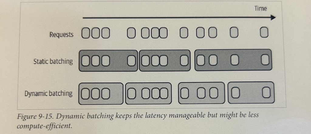
Continuous Batching: Allows responses in a batch to return to users as soon as they complete. Completed responses return immediately, and new requests can be processed in their place. This provides the best balance between throughput and latency.
Decoupling Prefill and Decode
LLM inference consists of prefill (compute-bound) and decode (memory bandwidth-bound). Using the same machine for both causes them to inefficiently compete for resources, significantly slowing down both TTFT and TPOT.
The solution: separate machines handle prefill and decode operations. Prefill instances use compute-optimized hardware, while decode instances use memory-optimized hardware. The ratio of prefill to decode instances depends on workload characteristics (longer inputs require more prefill compute) and latency requirements.
Prompt Caching
Prompt caching is invaluable for queries involving long documents or repeated system prompts.
Without prompt caching, your model processes the system prompt with every query. With prompt caching, the system prompt is processed once for the first query, then reused. Overlapping segments in different prompts can be cached and reused.
For applications with long system prompts, prompt caching can dramatically reduce both latency and cost.
Parallelism Strategies
Accelerators are designed for parallel processing, and parallelism strategies form the backbone of high-performance computing.
Replica Parallelism: The most straightforward strategy—simply creates multiple replicas of the model you want to serve. More replicas handle more simultaneous requests, potentially at the cost of using more chips.
Model Parallelism: Splits the same model across multiple machines. This becomes necessary when models don't fit on single machines.
Tensor Parallelism: Provides two benefits. First, it makes serving large models possible when they don't fit on single machines. Second, it reduces latency, though this benefit might be offset by extra communication overhead.
Pipeline Parallelism: Enables serving large models on multiple machines but increases total latency per request due to extra communication between pipeline stages. However, it's commonly used in training since it can increase throughput.
Context Parallelism: The input sequence itself is split across different devices for separate processing. For example, the first half of input processes on machine 1 and the second half on machine 2.
Sequence Parallelism: Operators needed for the entire input are split across machines. For example, if input requires both attention and feedforward computation, attention might process on machine 1 while feedforward processes on machine 2.
The Latency-Cost Trade-Off
AI applications face a fundamental latency/throughput trade-off. You can potentially reduce cost if you're okay with increased latency, and reducing latency often involves increasing cost.
The LinkedIn AI team's reflection after a year of deploying generative AI confirmed this: every optimization decision involves balancing these competing priorities based on your specific use case and user requirements.
Choosing the Right Optimization Techniques
The choice of optimization techniques depends entirely on your workloads:
KV caching is significantly more important for workloads with long contexts than short contexts
Prompt caching is crucial for workloads involving long, overlapping prompt segments or multi-turn conversations
Batching works better for workloads with predictable request patterns
However, across various use cases, the most impactful techniques are typically:
Quantization: Generally works well across models, reducing memory and increasing throughput
Tensor Parallelism: Both reduce latency and enable serving larger models
Replica Parallelism: Relatively straightforward to implement and scales horizontally
Attention Mechanism Optimization: Can significantly accelerate transformer models
Key Takeaways
A model's usability depends heavily on its inference cost and latency. Understanding and optimizing these factors separates successful production deployments from expensive experiments.
Critical insights to remember:
Inference dominates costs: While training gets attention, inference accounts for up to 90% of deployed AI system costs
Two distinct bottlenecks: Prefill is compute-bound, decode is memory bandwidth-bound—they require different optimization strategies
Metrics matter: TTFT, TPOT, throughput, and utilization metrics guide optimization decisions
Hardware constrains software: How efficiently models run depends fundamentally on underlying hardware
Model vs. service optimization: Model-level optimization changes behavior; service-level optimization changes how models are served
Context-specific choices: No one-size-fits-all solution—workload characteristics determine optimal techniques
The eternal trade-off: Latency and cost constantly push against each other
Conclusion
Inference optimization isn't glamorous, but it's essential. Every millisecond of latency reduction improves user experience. Every percentage point of throughput increase reduces costs. Every optimization decision compounds across millions of requests.
The field continues evolving rapidly. New hardware architectures emerge, novel algorithms are developed, and best practices constantly shift. But the fundamentals remain: understand your bottlenecks, measure what matters, choose optimizations matching your workload, and never stop iterating.
The difference between a proof-of-concept and a production system often comes down to inference optimization. Master these techniques, and you'll build AI applications that aren't just impressive demos—they're sustainable, cost-effective systems that deliver value at scale.
In the end, making AI models better, cheaper, and faster isn't just about technology—it's about making AI accessible, practical, and valuable for real-world applications. That's the promise of inference optimization, and it's a promise worth pursuing.